Go is hard not only because the rules are intricate, but because an empty board already offers hundreds of nearly interchangeable legal points. Exhaustive search to the end is impossible, and hand-written evaluators are easy to get wrong. MCTS charts a practical middle path: many random games, with compute steered toward more promising branches.
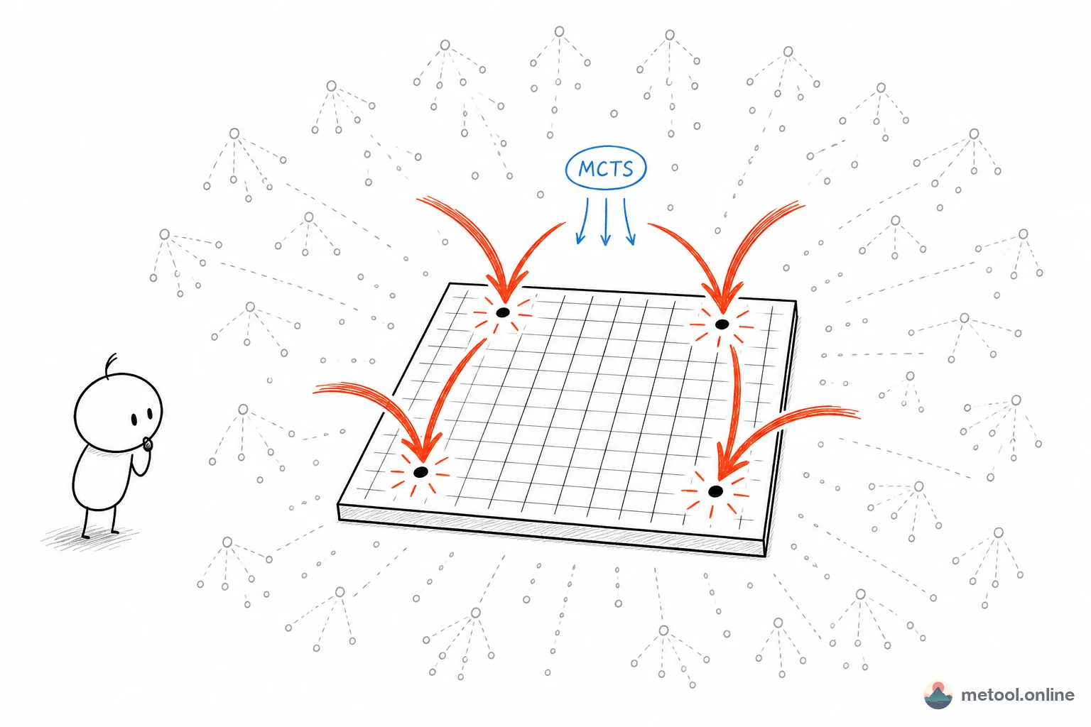
Why Is Go Especially Suited to—and Dependent on—MCTS?
Go's search space is too large to "calculate to the end": an empty 19×19 board has about 361 empty intersections, legal moves shift with the position, and games often run past a hundred moves. If each turn still has dozens of reasonable candidates, both width and depth explode. Hand-written heuristics (capture first, take corners, connect liberties) often degrade into aimless crawling along the edge in open openings.
MCTS (Monte Carlo Tree Search) does not try to exhaust the tree, and it does not rely on a global scoring table. It repeatedly plays short random games, backs up wins and losses, and spends more simulation budget on branches that look better. The larger the branching factor and the harder it is to write an accurate evaluator, the more valuable this "sample instead of exhaust" idea becomes—which is why it caught on in Go and later in many imperfect-information games.
What Does One MCTS Iteration Do?
A full MCTS iteration usually has four steps, repeated until time or simulation count runs out:
- Selection: From the root, walk down expanded children with a formula such as UCB1, balancing "known high win rate" against "not tried enough yet";
- Expansion: When a node still has untried legal moves, pick one (randomly or with a prior) and grow a new child;
- Simulation / Rollout: From the new position, both sides play randomly (or with a weak heuristic) to the end and score under the rules;
- Backpropagation: Write that game's result back along the path into each node's visits / wins.
The move finally played is usually the root child with the most visits (argmax visits), not the one with the highest instantaneous win rate—visit count already encodes "tried many times and still standing," which is stabler than early, noisy win rates.
| Step | Input | Output | Common pitfall |
|---|---|---|---|
| Selection | Expanded tree + UCB1 | Path to a leaf / node to expand | Exploration constant too high → flat visits |
| Expansion | Untried legal moves | One new child | Suicide / eye-fill at the root poisons the endgame |
| Simulation | Current position | One game outcome | Filling own eyes during rollouts corrupts value |
| Backprop | Outcome | Updated visits/wins on the path | Keep the perspective fixed (always relative to the same side) |
How Does UCB1 Trade Off Exploitation and Exploration?
UCB1 scores each child roughly as:
[ \frac{w_i}{n_i} + C \sqrt{\frac{\ln N}{n_i}} ]
The first term is empirical win rate (exploitation); the second grows when a node has been visited little (exploration). Larger (C) means more willingness to try unfamiliar branches.
Textbooks often set (C=\sqrt{2}\approx 1.41), derived for rewards in ([0,1]) with not too many children. A Go root often has dozens or hundreds of legal points, while a browser think may only run thousands to tens of thousands of simulations: the exploration term easily swamps win-rate gaps, so visits become almost uniform and the top move can fall to about 2%—poor move choice and unreadable "tendency" at the root. In practice (C) is often lowered (e.g. to 0.4) so a limited budget concentrates faster.
A useful convergence signal is the root top-1 visit share. On the same 9×9 position, ~1200 simulations often leave top-1 in the single-digit percent range; ~20,000 can reach about 17%; ~40,000 about 40%. When the share is low, prefer "not enough search" over "every point on the board is equally good."
How Do "Tendency" Scores Relate to the Move Played?
Each root child's visits / Σvisits can be read as relative tendency: where search spent compute. A UI that shows top-N candidates usually sorts by visits and truncates; the move played is still the visits maximum.
Boundaries that are easy to miss:
- Displayed probabilities often sum to less than 1: after filtering the long tail, the shown set need not sum to 1—on purpose. Top-1 share itself says how sure the search is;
- Too few simulations → flat distribution: thousands of playouts spread across a hundred empties on 19×19 leave only dozens of visits per point—tendency is near noise;
- Do not weaken play with temperature sampling on an unconverged distribution: sampling by visits when the distribution is still flat pushes it toward uniform and collapses into random play. A cleaner way to weaken is fewer simulations, still picking argmax.
Why Can't You Speed Up the Opening by "Thinking Less"?
An empty board has the most legal points and the fewest simulations per point—globally the hungriest stage for compute. A tempting reading: "Opening top-1 is only a few percent, so points are similar—search less." Self-play disagrees: the side that cuts opening budget against the same-strength engine can lose about 2:8. The right reading is low share = not converged yet, not "already equivalent."
A safer speedup is opening knowledge that narrows root candidates: restrict untried moves at the root to a few well-established points (e.g. still-empty corner star points). Branching drops from hundreds to a handful, and each candidate can get hundreds of simulations. When corners are taken, contact starts near those points, or a group drops to one liberty, fall back to full-board search. On large boards this usually saves time and raises per-point signal; on 9×9, where branching is already modest, forced narrowing can be a net loss—gate by board size.
Why Explicitly Avoid Filling Your Own Eyes in the Endgame?
Playing in your own true eye is usually legal but terrible—it kills liberties. If random rollouts fill eyes freely, valuations are polluted by self-destruction. If the root does not exclude own eyes, a side with nothing left to play may fill an eye and kill a living group instead of passing.
A more mature pure-MCTS Go engine handles both places: rollouts skip eye fills; root candidates filter own eyes. When only eye fills remain, the correct action is pass, so both sides can move into scoring.
Where Are the Limits of Pure MCTS?
Boundaries matter more than memorizing the formula:
| Dimension | Pure MCTS (random rollouts) | MCTS with policy/value nets |
|---|---|---|
| Prior | Almost none; concentrate via visits | Network move priors + position value |
| Strength at equal time | Hard-capped by sim count; noisy on large boards | Usually much stronger |
| Readable "tendency" | Directly from visit shares | Mixed with network prior—read separately |
| Implementation / compute | Feasible in a browser Web Worker | Needs model weights and more compute |
| Weakening difficulty | Lower maxSims / time |
Also tune temperature, noise, etc. |
A few more engineering boundaries: without a network, short 19×19 searches yield tendency that is reference-only; Chinese area scoring and Japanese territory scoring define different terminals—playout scoring must match product rules; ko and suicide legality must be correct in move generation, or the tree learns illegal shortcuts.
Takeaway
MCTS spends limited compute on more promising branches via selection → expansion → simulation → backprop, and usually plays the most-visited move. On Go's wide root, the UCB1 exploration constant, whether to narrow opening candidates, and whether rollouts forbid eye fills decide strength and readability under real budgets. When you read visit shares, ask first how many simulations ran—before convergence, a flat distribution means too little compute, not that every empty point is a good move.